


 161 / 372

臺大管理論叢
第
26
卷第
2
期
161
where
t
p
x
(
t
–1
p
x
) denotes the probability that an individual aged
x
will survive to age
x
+
t
(
x
+
t –
1);
q
x+t
–1
represents the probability that an individual aged
x
+
t –
1 will die within the
next year;
for
j
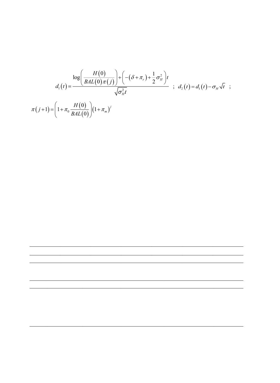
= 0,1,2,... .; and Φ is the cumulative distribution
function of the standard normal distribution.
The profits of the lender can be obtained by subtracting the loan amount, the value of
rental income, the remaining value, insurance premiums (expenses) from the property value,
plus the lender’s gain from RM insurance (the cost of RM insurance).
3. Findings
Table 1 lists the parameter assumptions for the numerical illustration. This study first
determines the maximum loan-to-value (LTV) ratio, and hence the maximum loan amount,
under which the present value of insurance premiums equals the cost of RM insurance. Table
2 lists the maximum loan amounts for borrowers in several age groups. We then examine the
sensitivity of the maximum loan amount to changes in certain key variables (see Table 3) for
a male borrower aged 70 years old.
Table 1 Parameter Assumptions
Parameter
H
(0)
δ
π
r
π
0
π
m
σ
H
Value
1,000,000
2%
1.5%
2% 1.25% 10.42%
Table 2 Maximum Loan Amounts for Borrowers of Different Ages
Age Loan Amount
Rental Income Remaining Value Insurance Expenses
Profits
62
307,357
336,570
201,947
141,865
154,126
65
345,237
304,852
203,771
134,872
146,140
70
414,290
252,204
203,591
120,765
129,915
75
487,218
202,917
198,444
104,756
111,420
80
561,994
158,098
188,080
87,829
91,829
Note: The profit of the lender is obtained by subtracting the former three components from
H
(0).