Page 50 - 34-1

Valuation of Spread and Basket Options

Appendix C. Derivation of Theorem 1

Appendix C. Derivation of Theorem 1
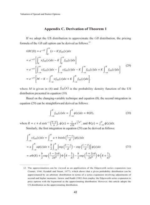
If we adopt the US distribution to approximate the GB distribution, the pricing
Appendix C. Derivation of Theorem 1
If we adopt the US distribution to approximate the GB distribution, the pricing formula of the GB call option
12
Appendix C. Derivation of Theorem 1
formula of the GB call option can be derived as follows:
If we adopt the US distribution to approximate the GB distribution, the pricing formula of the GB call option
12
can be derived as follows:
If we adopt the US distribution to approximate the GB distribution, the pricing formula of the GB call option
12
can be derived as follows:
Appendix C. Derivation of Theorem 1

�
can be derived as follows: 12 ��� � ( − (
(0

�
���pproximate the GB distribution, the pricing formula of the GB call option
If we adopt the US distribution to a � ( − (
��

(0
�
�
can be derived as fo ��� � � ( − ( ��
(0 llows:
12
�
�� �
��� �� ( − � ( �
�
�
�
�� �
Appendix C. Derivation of Theorem 1
��
���
(0 � ��� � ( − (
�� ( − � ( �
�
�
� ��
(29)

�� ( − � ( �
��
��
���
�

(29)
If we adopt the US distribution to approximate the GB distribution, the pricing formula of the GB call option
�
�
�
��
� ��
�
�
�
�
�
�
��� �� ( − � ( − � ( � ( � (29)
12
��� ( − � ( �
�
��
�
��
��
�� �
�
���
�� ( − � ( − � ( � ( �
can be derived as follows: �� ��� �� � �� �� � �� � �� (29)
��� �� ( − � ( − � ( � ( � ��
�
��
��
��
�
�
�
��
��
�
��
��
��
��( � ( �,
�
(0 ��� � � ( − ( �� �� � �� �� � �� (29)
��
���
��

�ℳ − − �
��
��
�
�
��� �� � ( − � ( − � ( � ( �
�
�
��
��
��
��
��
��
���
��
� − − � ( � ( �, � ( �, ��
��� �ℳ �� �ℳ − − � ( �� ��

��
�
��
��
where M is given in (4) and ( �
�
is the probability density function of the US
��
��� �� ( − � �� �� � ��
�ℳ − − � ( � ( �,
where ℳ is given in (4) and ( is the probability density function of the US distribution presented in
��
��
���

��
��
�
��
�
distribution presented in equation (10).
equation (10).
��
��
(29)
where ℳ is given in (4) and ( is the probability density function of the US distribution presented in
�� in (4) and ( is the probability density function of the US distribution presented in
where ℳ is given
�
�
�
�

Based on the changing-variable technique and equation (8), the second integration in
Based on the changing-variable technique and equation (8), the second integration in equation (29) can be
��
equation (10). ��� �� ( − � ( − � ( � ( �
equation (10).
��
��
��
��
�� in (4) and ( is the probability density function of the
straightforward derived as follows.
where ℳ is given �� �� �� ��US distribution presented in
equation (29) can be straightforward derived as follows:
Based on the changing-variable technique and equation (8), the second integration in equation (29) can be
Based on the changing-variable technique and equation (8), the second integration in equation (29) can be
equation (10). � � � �

straightforward derived as follows. � ( � ( Φ( , (30)
straightforward derived as follows.
�ℳ − − � ( � ( �,
���

��
Based on the changing-variable technique and equation (8), the second integration in equation (29) can be
��
��
�
�

��
��
(30)
�
straightforward derived as follows. �� �� � �� � (30) (30)
� ( � ( Φ( ,
��
� ( � ( Φ( ,
�

��
�
where sinh −1 � ��� �, ( � � � , and Φ( � � ( .
��
��
�� � ( � ( Φ( ,
� � �� �� (30)
��
√��
Similarly, the first integration in equation (29) can be derived as follows.
( .
��
where ℳ is given in (4) and ( is the probability density function of the US distribution presented in
�
���
�
�
−1
�
where sinh
�
, and Φ( �
where
�� �
( .
�
�, ( �����
�
��
�
�� −1
��
√��

�
� �
, and Φ( �
� sinh
where
�, (
�
equation (10). � ( � sinh � � − � ( � � ( .
Similarly, the first integration in equation (29) can be derived as follows.
��
√��
�
�� �
���
�
�
−1
Similarly, the first integration in equation (29) can be derived as follows:
where sinh

�, (
, and Φ(
�
� Similarly, the first integration in equation (29) can be derived as follows.
��

Based on the changing-variable technique and equation (8), the second integration in equation (29) can be
��
√��
� �

−
Similarly, the first integration in equation (29) can be derived as follows.
��
��
� (

�
�
� ( � sinh �
−
��
�
� (

�
straightforward derived as follows. � � − − �� ( (31)
�
�� ( � sinh �
��
−
��
� (
� ( � �exp � � − exp �

�
�
2 sinh �
� ( �
�
�
��
��
��
�� −
−
�� � ( � ( Φ( , (31) (30)

��
��
� ( � �exp �� � � � − exp � �� (
�

2 1−2 1 − 1 2 − 1 (31)
�� (
�� �
�
��
��
��
−
� −
Φ( exp � � Φ � − � − exp � − exp � � Φ � �. (31) (31)
� ( � �exp �

2
�
� ( 1−2 � 2 �� � 1 � − exp � 2 ( 1
2 � �exp �
��
2

1 2

( . �.
−1 ��� �� 2 � � �� �
�
2 � 2 √�� 1−2 2 1 2 � �� 1 2 1
where sinh exp � �� � , and Φ( � � Φ �
��
�, ( � Φ � − � − exp �
Φ(
�

� Φ � �.

1
1−2

1
1 2
With equations (29), (30), and (31), the pricing formula of the GB
� Φ � − � − exp �
Φ( exp �
� �.
Similarly, the first integration in equation (29) can be derived as follows. call option can be obtained. The
� Φ �
Φ( exp �
� − � − exp �
� Φ �

2
2

2
derivation of the pricing formula for the GB put option is similar to the call option and thus it has been omitted.
2 �
�
2
2
2
2

With equations (29), (30), and (31), the pricing
− formula of the GB call option can be obtained. The
�
�

� (

� ( � sinh �
derivation of the pricing formula for the GB put option is similar to the call option and thus it has been omitted.
��
��(29), (30), and (31), the pricing formula of the GB call option can be obtained. The
�� With equations

With equations (29), (30), and (31), the pricing formula of the GB call option can be obtained. The
derivation of the pricing formula for the GB put option is similar to the call option and thus it has been omitted.
12
� The approximation can be viewed as an application of the Edgeworth series expansion (see

�
(31)
−
−
derivation of the pricing formula for the GB put option is similar to the call option and thus it has been omitted.
�� (
Cramér, 1946; Kendall and Stuart, 1977), which shows that a given probability distribution can be

� ( � �exp �
� − exp �
�� approximated by an arbitrary distribution in terms of a series expansion involving adjustments of

2

second and higher moments. Jarrow and Rudd (1982) first employ the Edgeworth series expansion to
��
1−2 1 1 2 1

price options with the lognormal as the approximating distribution. However, this article adopts the
Φ( exp � � � Φ � − � − exp � � � Φ � �.

2
2
2
US distribution as the approximating distribution. 2

12 The approximation can be viewed as an application of the Edgeworth series expansion (see Cramér, 1946; Kendall and Stuart,

With equations (29), (30), and (31), the pricing formula of the GB call option can be obtained. The
42
1977), which shows that a given probability distribution can be approximated by an arbitrary distribution in terms of a series
12 The approximation can be viewed as an application of the Edgeworth series expansion (see Cramér, 1946; Kendall and Stuart,
derivation of the pricing formula for the GB put option is similar to the call option and thus it has been omitted.
expansion involving adjustments of second and higher moments. Jarrow and Rudd (1982) first employ the Edgeworth series expansion

1977), which shows that a given probability distribution can be approximated by an arbitrary distribution in terms of a series

to price options with the lognormal as the approximating distribution. However, this article adopts the US distribution as the
expansion involving adjustments of second and higher moments. Jarrow and Rudd (1982) first employ the Edgeworth series expansion Stuart,
12 The approximation can be viewed as an application of the Edgeworth series expansion (see Cramér, 1946; Kendall and
approximating distribution.
12 The approximation can be viewed as an application of the Edgeworth series expansion (see Cramér, 1946; Kendall and Stuart,
1977), which shows that a given probability distribution can be approximated by an arbitrary distribution in terms of a
to price options with the lognormal as the approximating distribution. However, this article adopts the US distribution as the series
1977), which shows that a given probability distribution can be approximated by an arbitrary distribution in terms of a series
expansion involving adjustments of second and higher moments. Jarrow and Rudd (1982) first employ the Edgeworth series expansion
approximating distribution. 38
expansion involving adjustments of second and higher moments. Jarrow and Rudd (1982) first employ the Edgeworth series expansion
to price options with the lognormal as the approximating distribution. However, this article adopts the US distribution as the
to price options with the lognormal as the approximating distribution. However, this article adopts the US distribution as the
approximating distribution. 38
approximating distribution.
38
38

12 The approximation can be viewed as an application of the Edgeworth series expansion (see Cramér, 1946; Kendall and Stuart,
1977), which shows that a given probability distribution can be approximated by an arbitrary distribution in terms of a series
expansion involving adjustments of second and higher moments. Jarrow and Rudd (1982) first employ the Edgeworth series expansion
to price options with the lognormal as the approximating distribution. However, this article adopts the US distribution as the
approximating distribution.
38