Page 37 - 34-1

NTU Management Review Vol. 34 No. 1 Apr. 2024

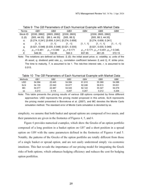
Table 9 The GB Parameters of Each Numerical Example with Market Data
Terms GB1 GB2 GB3 GB4 GB5 GB6
Stock ID [2330, 2882] [2603, 2882] [2330, 2603] [2330, 2603, 2882]
S i (0) [505, 44.55] [88.3, 44.55] [505, 88.3] [505, 88.3, 44.55]
[0.274, 0.241] [0.658, 0.241] [0.274, 0.658] [0.274, 0.658, 0.241]
σ i
[1, 1] [1, 1] [1, -1] [1, 1, 1] [1, -1, 1] [1, -1, -1]
α i
[0.021, 0.048] [0.035, 0.048] [0.021, 0.035] [0.021, 0.035, 0.048]
q i
ρ 1,2 = 0.451 ρ 1,2 = 0.340 ρ 1,2 = 0.171 ρ 1,2 = 0.171, ρ 1,3 = 0.451, ρ 2,3 = 0.340,
ρ i,j
K 549.55 132.85 593.3 637.85 461.25 372.15
Note: The notations are defined as follows: S i (0): the initial asset price; σ i : volatility; α i : units of the
ith asset; q i : dividend yield rate; ρ i,j : correlation coefficient between S i and S j ; K: strike price.
The time to maturity, T, is assumed to be 1. The risk-free interest rate, r, is assumed to be
0.015.

Table 10 The GB Parameters of Each Numerical Example with Market Data
Methods GB1 GB2 GB3 GB4 GB5 GB6
USD 54.094 22.445 54.584 61.910 55.368 54.086
SLN 54.155 23.540 55.977 62.246 56.615 55.631
MC 54.077 22.487 54.543 62.122 55.327 54.079
se 0.213 0.114 0.207 0.247 0.212 0.204
Note: This table presents the pricing results of various GB options computed by three different
approaches: USD represents the pricing model proposed in this article, SLN represents
the pricing model presented in Borovkova et al. (2007), and MC denotes the Monte Carlo
simulation method. The standard error of Monte Carlo simulation is denoted by se.

simplicity, we assume that both basket and spread options are composed of two assets, and
their parameters are given in the footnotes of Figures 4, 5, and 6.

Figure 6 provides numerical examples, which show the Greeks of an option portfolio
composed of a long position in a basket option on GB7 and a short position in a spread
option on GB8 with the same parameters defined in the footnotes of Figures 4 and 5.

Notably, the patterns of the Greeks of the option portfolio are totally different from those
of a single basket or spread option, and are not easily understood simply via economic
intuitions. This fact reveals the importance of our pricing model for integrating the Greek
risks of both options, which enhances hedging efficiency and reduces the cost for hedging
option portfolios.

29