Page 28 - 34-1

To evaluate the performance of each model by comparing it with the result computed based on the Monte
Valuation of Spread and Basket Options
To evaluate the performance of each model by comparing it with the result computed based on the Monte
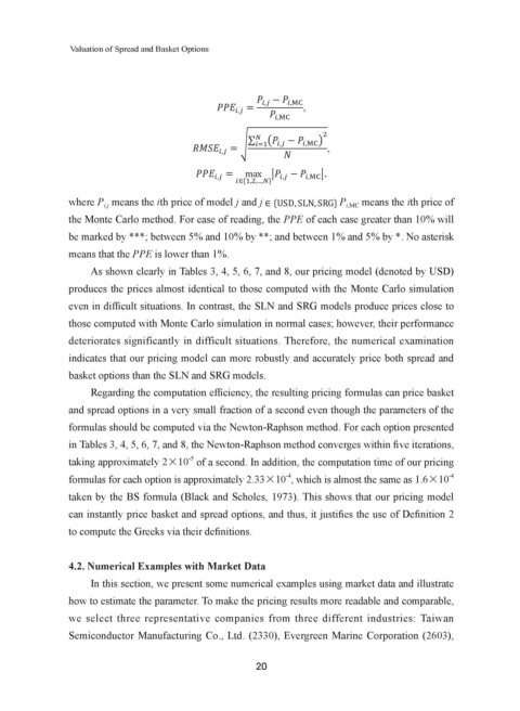
Carlo simulation method, we provide the percentage pricing error ( ), root of mean squared error ( ),
Carlo simulation method, we provide the percentage pricing error ( ), root of mean squared error ( ),
and maximum absolute error ( ), which are computed as follows:
and maximum absolute error ( ), which are computed as follows:
−
, ,
�,��
�,�
�,� = �,� − �,��
�,��
�,� = ,
�,��
�
∑ � � − �,�� �
� ��� �,� , , �
�,� = ∑ � � �,� − �,�� �
�,� = � ��� ,

�,� = max � − �,�� �. ,
�,�
� ��,�,...,�� max � − �,�� �.

=
�,�
� ��,�,...,�� �,�
where means the th price of model and �USD, SLN, SRG�. �,�� means the th price of the Monte Carlo
means the ith price of
where P means the ith price of model j and j . P
i,MC means the th price of the Monte Carlo
�,�
where means the th price of model and �USD, SLN, SRG�.
i,j �,�
�,��
method. For ease of reading, the of each case greater than 10% will be marked by ***; between 5% and
the Monte Carlo method. For ease of reading, the PPE of each case greater than 10% will
method. For ease of reading, the of each case greater than 10% will be marked by ***; between 5% and
10% by **; and between 1% and 5% by *. No asterisk means that the is lower than 1%.
be marked by ***; between 5% and 10% by **; and between 1% and 5% by *. No asterisk
10% by **; and between 1% and 5% by *. No asterisk means that the is lower than 1%.
As shown clearly in Tables 3, 4, 5, 6, 7, and 8, our pricing model (denoted by USD) produces the prices
As shown clearly in Tables 3, 4, 5, 6, 7, and 8, our pricing model (denoted by USD) produces the prices
means that the PPE is lower than 1%.
almost identical to those computed with the Monte Carlo simulation even in difficult situations. In contrast, the
almost identical to those computed with the Monte Carlo simulation even in difficult situations. In contrast, the
As shown clearly in Tables 3, 4, 5, 6, 7, and 8, our pricing model (denoted by USD)
SLN and SRG models produce prices close to those computed with Monte Carlo simulation in normal cases;
SLN and SRG models produce prices close to those computed with Monte Carlo simulation in normal cases;
produces the prices almost identical to those computed with the Monte Carlo simulation
however, their performance deteriorates significantly in difficult situations. Therefore, the numerical
however, their performance deteriorates significantly in difficult situations. Therefore, the numerical
even in difficult situations. In contrast, the SLN and SRG models produce prices close to
examination indicates that our pricing model can more robustly and accurately price both spread and
examination indicates that our pricing model can more robustly and accurately price both spread and basket basket
those computed with Monte Carlo simulation in normal cases; however, their performance
options than the SLN and SRG models.
options than the SLN and SRG models.
deteriorates significantly in difficult situations. Therefore, the numerical examination
Regarding the computation efficiency, the resulting pricing formulas can price basket and spread options in
Regarding the computation efficiency, the resulting pricing formulas can price basket and spread options in
indicates that our pricing model can more robustly and accurately price both spread and
a very small fraction of a second even though the parameters of the formulas should be computed via the
a very small fraction of a second even though the parameters of the formulas should be computed via the
basket options than the SLN and SRG models.
Newton-Raphson method. For each option presented in Tables 3, 4, 5, 6, 7, and 8, the Newton-Raphson method
Newton-Raphson method. For each option presented in Tables 3, 4, 5, 6, 7, and 8, the Newton-Raphson method
�� × 10 of a second. In addition, the computation time
Regarding the computation efficiency, the resulting pricing formulas can price basket
��
converges within five iterations, taking approximately 2
converges within five iterations, taking approximately 2 × 10 of a second. In addition, the computation time
of our pricing formulas for each option is approximately 2.33 × 10 , which is almost the same as 1.6 × 10
and spread options in a very small fraction of a second even though the parameters of the
��
of our pricing formulas for each option is approximately 2.33 × 10 , which is almost the same as 1.6 × 10 ��
��
��
taken by the BS formula (Black and Scholes, 1973). This shows that our pricing model can instantly price
formulas should be computed via the Newton-Raphson method. For each option presented
taken by the BS formula (Black and Scholes, 1973). This shows that our pricing model can instantly price
basket and spread options, and thus, it justifies the use of Definition 2 to compute the Greeks via their
basket and spread options, and thus, it justifies the use of Definition 2 to compute the Greeks
in Tables 3, 4, 5, 6, 7, and 8, the Newton-Raphson method converges within five iterations, via their
definitions.
taking approximately 2×10 of a second. In addition, the computation time of our pricing
definitions. -5

-4
formulas for each option is approximately 2.33×10 , which is almost the same as 1.6×10
-4

taken by the BS formula (Black and Scholes, 1973). This shows that our pricing model

can instantly price basket and spread options, and thus, it justifies the use of Definition 2

to compute the Greeks via their definitions.

4.2. Numerical Examples with Market Data
In this section, we present some numerical examples using market data and illustrate
how to estimate the parameter. To make the pricing results more readable and comparable,
we select three representative companies from three different industries: Taiwan
17

Semiconductor Manufacturing Co., Ltd. (2330), Evergreen Marine Corporation (2603),
17

20