Page 23 - 34-1

method and shows the sufficient conditions for convergence. Therefore, we adopt the method proposed by
method and shows the sufficient conditions for convergence. Therefore, we adopt the method proposed by Tuenter
Tuenter (2001) to solve equation (16), and arrange and reduce their results into the following three steps.
(2001) to solve equation (16), and arrange and reduce their results into the following three steps.
NTU Management Review Vol. 34 No. 1 Apr. 2024
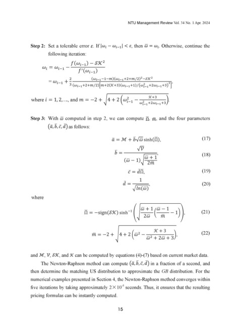
Step 1: Compute the initial value ω as follows:
method and method and shows the sufficient conditions for convergence. Therefore, we adopt the method proposed method and method and shows the sufficient conditions for convergence. Therefore, we adopt the method proposed by by shows the sufficient conditions for convergence. Therefore, we adopt the method proposed by by
�
h

e
e
b
m
e
u
sthe
c

n
y
hodethod
refore, refore,
T
t
o
h
e
h
sand
wshows

T
.
t
h
e

s
f
r
p
posedposed
n
cfor
c
o

o
i
s
o
n
dconditions
f
t
i
o
csufficient
r
e

f

i
g
i
t
nvconvergence.

ro
p
e
n
ro
we
e
pt adopt
e
method
do
awe
th
mthe

Step 1: Compute the initial value ω as follows:

�
Tuenter (2001) Tuenter (2001) to solve equation (16), and arrange and reduce their results into the following three steps. Tuenter (2001) to solve equation (16), and arrange and reduce their results into the following three steps. eps.
ts int
heir r
owi
owi
eps.
e foll
lv
o so
o so
01)
t
ng three st

t
t
1

on
e foll
l
e equ
o th
g
(
√ − −

a
t
e and reduce
t
6
), and arran
esu
Tuenter
e and reduce
(2
on
ng three st
ts int
lv
i
l

Tuenter (2001) to solve equation (16), and arrange and reduce their results into the following three steps.
heir r
o th
0
), and arran

1
esu
g
i
(
a
e equ
t
6
�

ω =
�
Step 1: Compute the initial value ω as follows: as follows:
it
St
t

1
he i
ep
i
Step 1: Compute the initial value ωal value ω as follows: � � √ − − . Otherwise, continue the
te
Compu
n
:
Step 2: Set a tolerable error . If
, then
ω =
Step 1: Compute the initial value ω
Step 1: Compute the initial value ω as follows: as follows: ��
�
�
�
Step 2: Set a tolerable error . If | − ��� | < , then � = . Otherwise, continue the following
�
�
following iteration: | < , then � = . Otherwise, continue the following iteration:
iteration: Step 2: Set a tolerable error . If | − ω =− − √ − − − − − �
�
���
� �
� �
√ ω = �
√
ω
ω = = ω =
√ −
√ − −
� �
� �
( � ��� � � �
� −
) −
| < , then � = , then � = . Otherwise, continue Otherwise, continue the following
| < , then � then � = . Otherwise, continue the following
Step

t
Step 2: Set Step Step 2: Set 2: aSet = a tolerable error . If | − − − � � | < , | < , then � = . Otherwise, continue the following . Otherwise, continue the following the following .
− . If | .
���
Step ole 2: Set a tolerable error
| < =
= a tolerable error
� 2: Set a rable error . If | � If |
���
�
�
����
�
�
� ��� − ���tolerable error . If | − − ��� ��� ��� � � � � �
�
)
(
���
iteration:
iteration:
iteration:
iteration: iteration: � ��� �� ��� ������� ��� ���� �� � �
�
� ,
�
⁄ �
(� ��� ����)(� ��� ���� �) �
�
⁄
�
=

= ��� ( ��� ( � �� ��� ���� ������� ����� ��� ��� �� � ��� ��� ��� �

� �
� �
���
�
)
)
)) −
(
) − ( − −
⁄ −
⁄

�
⁄ ���
� (� ��� ���� �)����( ��)(� ��� ��) ��
��� ��� �
= − = − ��� ��� ( ��� ⁄ ��� ��� ���
− −
� � =
� � −
= ��� = ��� � �
���
���
�
� �
) )
��� �
)
( ��� ( ��� ( ( ��� ))
(
���
���
� �� �� �.
�.
− � �
� �
� �
� �
�
where = , and = − �4 � �
⁄ ⁄
where = , and = − �4 � ���� �))(� (� ��� ����)(� ��� ���� �) � � � (� � ����)(� ��� ���� �) � � � − ⁄ ⁄ ��� � � ��� ��
�
�
⁄
(� ��� ����)(� ������ ���� �) � ���� �) �
��� ��� ��
� ��� ��������)(� ���
(� ���(� ���
=

= = ��� � �
= ��� = ��� � � ��� ��� � �
��� ��� � (� ��� ⁄ �)����( ��)( ⁄ ⁄ � � ��� ��� ��� ��� ��� �
���
���
� �
�
�
⁄� �
��� ��� ��
��� ��� ��� � �
��� ��� ���
� (� ��� ����
⁄ �)����( ��)(� ��� ��) ��� ��� ��) �� ��)⁄
⁄
� (� ��� ���� �)����( ��)(� ��� ��) �����( ��)(� ��� ��) �� ��� ��
Step 3: With � computed in step 2, we can compute Ω, �, and the four parameters � � ̅ � as follows:
⁄ ��� � ���
� (� ��� ���� �)� (� ��� ����⁄⁄ ���� �)����( ��)(� ���
���
���
���
�
�
̅
Step 3: With � computed in step 2, we can compute Ω, �, and the four parameters � � ̅ � as follows:
̅
�
�
−�.
,
��
d
an
an
,
d
��
Step 3: With computed in step 2, we can compute , , and the four parameters
− �.
��
��
� �
− −
� = ℳ √ � sinh�Ω� ��� ��� ����� ��� ��� ��� �� ��� ��� �� (17)

−
4 �

where
where = , and = − �4 −
=
where = where = , and = − �4 where = , and = − �4 � � � � � � � � �� � � � �. �. �. (17)

−
=

4
�

=

�
� �
���
���
���
�
���
��� ��
� � �
��� �
��� �
��� ���
� ���
as follows: � = ℳ √ � sinh(Ω) ������ ���
Step 3: With
Step 3: With � computed in step 2, we can compute Ω, �, and the four parameters � � ̅ � as follows: � computed in step 2, we can compute Ω, �, and the four parameters � � ̅ � as follows:
Step 3:
√ � �

� �
� �
��
Step 3: With Step 3: With � computed in step 2, we can compute Ω, �, and the four parameters � � ̅ � as follows: � computed in step 2, we can compute Ω, �, and the four parameters � � ̅ � as follows: With � computed in step 2, we can compute Ω, �, and the four parameters � � ̅ � as follows:
̅ ̅
̅
̅̅ �
�

√
�

(18)
=
�
=
� = ℳ √ � = ℳℳ √ √ � sinh � � � (17) (17) (18) (17)
(17)
(17)
� � − �� sinh(Ω) Ω) √ � sinh(Ω) ,
� = ℳ � sinh( � � sinh(Ω) (Ω)
� �
�
�
�� �
� = � = ℳ
( � − )� � √ � �
√ √ �
√ √
√
(19)

= = = = = ̅ = Ω � , (18) (18) (19) (18)
�
�
(18)
�
(18)
�
�
̅ = Ω
̅�
̅�
�
�
� �
( � − )�
( � − )�
( �
( � − )� − ) ( � − )�� � � � (20)
� �

̅

=
̅
=
(19)
̅ = Ω = Ω ̅ = Ω ̅ ���� �� (19) (19) (20) (19)
(19)
���( �) = ٠,
̅� ̅�
̅� ̅�
̅ = Ω ̅�
̅
where

where ̅ ̅ ̅ = = , (20) (20) (20)

(20)
̅
(20)

̅
= = = ���( �) �)
���(
���( �) �) �)
���( ���(
� � −
− ��
− � � −
�
where
where
where where where Ω = −sign( ) sinh − �� �� � � − �� (21) (21)

Ω = −sign� � sinh
�
� � � �

�
(21)
�
(21)
− ��
Ω = −sign( ) − �� � � � − � � − � − � � � − � − � − − �� , (21) (21) (21)
�� − �� � ��
− −
−
�
�
−
�
�
��
� �� − ��
�
� Ω = −sign( )
� Ω = −sign( ) sinhsinh
Ω = −s
Ω = −sign( ) sinhsinhign( ) sinh

� 3 � �
�
� � � � � � � 3 � (22) (22)
� = − �4 � � − �
�
� = − �4 � � − � � � 3
�
� � 3
(22)
3 3
(22) (22)
and ℳ, , , and can be computed by equations (4)-(7) based on current market data. (22)

3 3 3
and ℳ, , , and can be computed by equations (4)-(7) based on current market data. (22)
� � ,
� � �
� �
� �
�

� = − � �
� = −
� = − �4 � � −− �4 � � −− � � −
� = − �4 � � � = − �4 �4
� �
� �
� � 3 3
�
�
� � 3 � � � � 3 � 3
The Newton-Raphson method can compute � � ̅ � in a fraction of a second, and then determine the
�
̅
The Newton-Raphson method can compute � � ̅ � in a fraction of a second, and then determine the
�
̅
and ℳ, , , and
and ℳ, , , and can be computed by equations (4)-(7) based on current market data. can be computed by equations (4)-(7) based on current market data.
and ℳ, , , and , and

a
,
,
nd
and ℳ, , , and can be computed by equations (4)-(7) based on current market data. can be computed by equations (4)-(7) based on current market data. can be computed by equations (4)-(7) based on current market data.
matching US distribution to approximate the GB distribution. For the numerical examples presented in Section 4,
ℳ

matching US distribution to approximate the GB distribution. For the numerical examples presented in Section
, ,
and
, and can be computed by equations (4)-(7) based on current market data.
The Newton-Raphson method can compute � � ̅ � in a fraction of a second, and then in a fraction of a second, and then determine then in a fraction

an
omput
d
c
� ̅ � in a fraction of a second, and of a second, and then determine
c
The Newton-Raphson
�� determine the the determine the the the
The Newton-Raphson method can compute � � ̅ � � ̅ � in a fraction of a second, and then determine
The Newton-Raphson
�
�
̅ ̅
̅
̅̅ �
the Newton-Raphson method converges within five iterations by taking approximately × 0 seconds. Thus,
e �

The Newton-Raphson method can �
metho method can compute �
� compute � � ̅ �
0, the Newton-Raphson method converges within five iterations by taking approximately × 0 seconds.
��
in a fraction of a second, and
The Newton-Raphson method can compute
matching US matching US distribution to approximate the GB distribution. For the numerical examples presented in Section matching US distribution to approximate the GB distribution. For the numerical examples presented in Section
S
ist
n
the
e
r
.
i

al
e

F
n
e
butio
or
US
ibutio
F
ection
ist

i
d

to
c
xamples
pproximat
d
butio
matching US distribution to approximate the GB distribution. For the numerical examples presented in Section

xamples
esented
p
a
numeri
n
pproximat
istri
d
the
ibutio
ection
al
S
r
n
r
c
p
n
or
esented
numeri
to
the

e

istri

a
the
r
n
d
matching
.
B
B
G
G
it ensures that the resulting pricing formulas can be instantly computed.
Thus, it ensures that the resulting pricing formulas can be instantly computed.
then determine the matching US distribution to approximate the GB distribution. For the
ely
ap
s

ion
n
e
kin
t
r
etho
0, the Newton-Raphson method converges within five iterations by taking approximately × 0 seconds. seconds. 0 seconds. seconds.
ta
iv
co
ima
g
n
d
ox
f
0, the Newton
it
b
y

e
r
thi
ver
-
at
Raphson
wi
ges
p
m
ion
ta
ver
kin
y
s
he
t
r
ima
n
b
N
ewton

at
ely
ox
it

etho
0,
Raphson
thi
e
iv

m
g
ap
n
0, the Newton-Raphson method converges within five iterations by taking approximately × 0× 0 seconds.
co
p
ges
r
wi
d
-
f
e
t
�� ��
��
��
��
×
0

0, the Newton-Raphson method converges within five iterations by taking approximately ×

numerical examples presented in Section 4, the Newton-Raphson method converges within
Thus, it ensure Thus, it ensures that the resulting pricing formulas can be instantly computed. Thus, it ensures that the resulting pricing formulas can be instantly computed. ut e d .
in
for
p
Thus, it ensures that the resulting pricing formulas can be instantly computed.
e
c
c
resu
c
b
d
a
lt
g
e
r
in
c
p
ul
i
om
ut

p
in
n
as
m
c
lt
r
n
the
t
hat
hat
e
t
a
for
n
in
s
l
t
y
g
s
ul
c
t
a
p
t
n
in
l
nsure
Thus, it e
the
a
m
as
y
.
s
g
s
g
in
om

i
resu
t
b
3.2. Pricing Formula of the Basket/Spread Options with the US Distribution
five iterations by taking approximately 2×10 seconds. Thus, it ensures that the resulting
-5
3.2. Pricing Formula of the Basket/Spread Options with the US Distribution

Basket/Spread options are financial contracts on the basket/spread of multiple underlying assets whose final
pricing formulas can be instantly computed.
Basket/Spread options are financial contracts on the basket/spread of multiple underlying assets whose final
3.2. Pricin3.2. Pricing Formula of the Basket/Spread Options with the US Distribution 3.2. Pricing Formula of the Basket/Spread Options with the US Distribution
d
sk
et/Sp
f th

mula
istribution
istribution
o
e Ba
d
ea
r
f th
e Ba
ea
r
Optio

o
n
sk
o
et/Sp
g
ricin
3.2. Pricing Formula of the Basket/Spread Options with the US Distribution
g
s with the US D
F
r
n
o
r
Optio
3.2. P
s with the US D
mula
F
payoffs can be jointly defined as follows:
payoffs can be jointly defined as follows:
Basket/Spread Basket/Spread options are financial contracts on the basket/spread of multiple underlying assets whose final Basket/Spread options are financial contracts on the basket/spread of multiple underlying assets whose final fi nal
hose
nal
fi
ing
assets
ing
w
w
nderly
hose
assets
u
i
ont
ract
al
c
al
nan
c

on
s
t
ract
c

s
ont
i
a
opt
re
io
ns
Basket/Spread options are financial contracts on the basket/spread of multiple underlying assets whose final
Basket/Spread
io
opt
c
re
i
f
nan
f
ns
a
i
l
o
ti
f
mu
o
spr
f
ead
p
u
le
nderly
ti
p
mu
l
le
/

h
h
basket
e
on

spr
/
basket
e
ead

t 15
payoffs can be j payoffs can be jointly defined as follows: payoffs can be jointly defined as follows: 12 12
e
ointl
y d
payoffs can be j
payoffs can be jointly defined as follows:
ointl
e
ned as follows:
f
ned as follows:
i
y d
f
i

12
12 12 12 12