Page 24 - 33-3

Proof. Given any construction plan , each flow on the graph we constructed is
bounded by the demand of customers and capacity of facilities. Therefore, the capacity
constraints in benefit evaluation problem are obeyed. For every node , if the
�
Optimal Allocation of Capacitated Facilities Considering Time-Dependent User Preference for User Number
Maximization
maximum flow flows out according to the preference levels in equilibrium, the
customers’ decisions in graph are exactly the same as that in the benefit evaluation

problem. It turns out . Based on this maximum flow instance, assume

that there is at least one flow flowing out some node C changes to the less preferred
�
edge. If this change does not decrease , i.e., does not make any edge out of

capacity, . If it does, this new instance is impossible to be an outcome

of the maximum flow problem. In conclusion, even we allow the customers to choose

the facility which is not her/his most preferred in constructed maximum flow,

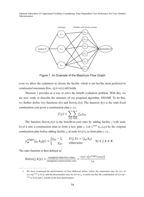
still holds. Figure 1 An Example of the Maximum Flow Graph

Theorem 1 provides us a way to solve the benefit evaluation problem. With this,
even we allow the customers to choose the facility which is not her/his most preferred in
constructed maximum flow, z(y)=w(y) still holds.
we are now ready to describe the structure of our proposed algorithm, GSAMF. To do
Theorem 1 provides us a way to solve the benefit evaluation problem. With this, we

this, we further define two functions and . The function
are now ready to describe the structure of our proposed algorithm, GSAMF. To do this, is
we further define two functions f(y) and Ratio(j,k|y). The function f(y) is the total fixed
the total fixed construction cost given a construction plan , i.e.,
construction cost given a construction plan y, i.e.,

� � .
�� ��
� � � �
The function Ratio(j,k|y) is the benefit-to-cost ratio by adding facility j with scale
The function is the benefit-to-cost ratio by adding facility with scale
origin
(j ,k |y) be the original
level k into a construction plan to form a new plan y. Let y
0
0
construction plan before adding facility j at scale level k to form plan y, i.e.,
level into a construction plan to form a new plan 0 . Let ������ be the
0
� �
original construction plan before adding facility at scale level to form plan ,
if (
) = (
)
− 1,
( ) � �
, otherwise
i.e.,
3
The ratio function is then defined as
The ratio function is then defined as 3
− 1 if
∀ .
������ �� � �
�� � �(�)���� ������ (� � �)�
������������������������
�
�
=
( ) = otherwise .
��
�������������������������� � ��
In each iteration of GSAMF, we are given an original construction plan. We test
3 We have examined the performance of four different ratios, where the numerator may be z(y) or
origin
(j,k|y)), and the denominator may be f(y) or f jk . It turns out that the combination of z(y)-z( y-
z(y)-z( y
each unbuilt facility with each candidate scale level by calculating the benefit-to-cost
22
origin
(j,k|y)) and f jk results in the best performance.

ratio upon adding it into the given construction plan. After choosing the one resulting
16
in the highest ratio, we proceed to the next iteration. We stop until all locations have
been chosen or we run out of budget. The pseudocode of the greedy selection algorithm
with maximum flow is presented in Algorithm 1.

3 We have examined the performance of four different ratios, where the numerator may be

( ) or ( ) − � ������ ( )�, and the denominator may be ( ) or . It turns out that the
��
������ ( )� and results in the best performance.
combination of ( ) − � ��
23