Page 121 - 臺大管理論叢第32卷第1期

out-of-sample once. Two quality indices are computed for model validation: Mean
out-of-sample once. Two quality indices are computed for model validation: Mean
Absolute Error (MAE) and the Root Mean Squared Error (RMSE). The MAE is equal to
Absolute Error (MAE) and the Root Mean Squared Error (RMSE). The MAE is equal to
the absolute difference between the actual value of gift giving and posting observed at
out-of-sample once. Two quality indices are computed for model validation: Mean
out-of-sample once. Two quality indices are computed for model validation: Mean
out-of-sample once. Two quality indices are computed for model validation: Mean
out-of-sample once. Two quality indices are computed for model validation: Mean
the absolute difference between the actual value of gift giving and posting observed at
time step t, throughout the duration of the lievestream, and the estimated gift-sending
Absolute Error (MAE) and the Root Mean Squared Error (RMSE). The MAE is equal to
Absolute Error (MAE) and the Root Mean Squared Error (RMSE). The MAE is equal to
Absolute Error (MAE) and the Root Mean Squared Error (RMSE). The MAE is equal to
Absolute Error (MAE) and the Root Mean Squared Error (RMSE). The MAE is equal to
time step t, throughout the duration of the lievestream, and the estimated gift-sending
value of the HB model at that same time step, and averaged overall values. RMSE is the
out-of-sample once. Two quality indices are computed for model validation: Mean
the absolute difference between the actual value of gift giving and posting observed at
the absolute difference between the actual value of gift giving and posting observed at
the absolute difference between the actual value of gift giving and posting observed at t
the absolute difference between the actual value of gift giving and posting observed a
value of the HB model at that same time step, and averaged overall values. RMSE is the
standard deviation of the average of squared differences between the estimated gift-
Absolute Error (MAE) and the Root Mean Squared Error (RMSE). The MAE is equal to
time step t, throughout the duration of the lievestream, and the estimated gift-sending
time step t, throughout the duration of the lievestream, and the estimated gift-sending
time step t, throughout the duration of the lievestream, and the estimated gift-sending
time step t, throughout the duration of the lievestream, and the estimated gift-sending
standard deviation of the average of squared differences between the estimated gift-
sending value and actual gift-sending value at time step t. We compute the MAE and
the absolute difference between the actual value of gift giving and posting observed at
value of the HB model at that same time step, and averaged overall values. RMSE is the
value of the HB model at that same time step, and averaged overall values. RMSE is the
value of the HB model at that same time step, and averaged overall values. RMSE is the
value of the HB model at that same time step, and averaged overall values. RMSE is the
sending value and actual gift-sending value at time step t. We compute the MAE and
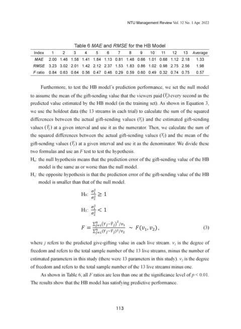
RMSE across all 13 trials for the HB model and compare the differences. The results
time step t, throughout the duration of the lievestream, and the estimated gift-sending
standard deviation of the average of squared differences between the estimated gif
standard deviation of the average of squared differences between the estimated gift-t-
standard deviation of the average of squared differences between the estimated gift-
standard deviation of the average of squared differences between the estimated gift-
RMSE across all 13 trials for the HB model and compare the differences. The results
are reported in Table 6. Details of the cross-validation MAE and RMSE are small. As
value of the HB model at that same time step, and averaged overall values. RMSE is the
sending value and actual gift-sending value at time step t. We compute the MAE and
sending value and actual gift-sending value at time step t. We compute the MAE and
sending value and actual gift-sending value at time step t. We compute the MAE and
sending value and actual gift-sending value at time step t. We compute the MAE and
are reported in Table 6. Details of the cross-validation MAE and RMSE are small. As
mentioned previously, we perform a log transformation for the variable of gift giving.
standard deviation of the average of squared differences between the estimated gift-
RMSE across all 13 trials for the HB model and compare the differences. The results
RMSE across all 13 trials for the HB model and compare the differences. The results
RMSE across all 13 trials for the HB model and compare the differences. The results
RMSE across all 13 trials for the HB model and compare the differences. The results
mentioned previously, we perform a log transformation for the variable of gift giving.
We use the exponential of the RMSE value to restore it to RMB. As shown in Table 6,
sending value and actual gift-sending value at time step t. We compute the MAE and
are reported in Table 6. Details of the cross-validation MAE and RMSE are small. As
are reported in Table 6. Details of the cross-validation MAE and RMSE are small. As
are reported in Table 6. Details of the cross-validation MAE and RMSE are small. As
are reported in Table 6. Details of the cross-validation MAE and RMSE are small. As
We use the exponential of the RMSE value to restore it to RMB. As shown in Table 6,
the RMSE value of the first trial is 3.23, so the exponential is 25.27 RMB. This shows
RMSE across all 13 trials for the HB model and compare the differences. The results
mentioned previously, we perform a log transformation for the variable of gift giving.
mentioned previously, we perform a log transformation for the variable of gift giving.
mentioned previously, we perform a log transformation for the variable of gift giving
mentioned previously, we perform a log transformation for the variable of gift giving. .
the RMSE value of the first trial is 3.23, so the exponential is 25.27 RMB. This shows
that our prediction error of the viewers’ gift-sending value in the 13th live stream is
are reported in Table 6. Details of the cross-validation MAE and RMSE are small. As
We use the exponential of the RMSE value to restore it to RMB. As shown in Table 6,
We use the exponential of the RMSE value to restore it to RMB. As shown in Table 6,
We use the exponential of the RMSE value to restore it to RMB. As shown in Table 6,
We use the exponential of the RMSE value to restore it to RMB. As shown in Table 6,
that our prediction error of the viewers’ gift-sending value in the 13th live stream is
25.27 RMB.
mentioned previously, we perform a log transformation for the variable of g
the RMSE value of the first trial is 3.23, so the exponential is 25.27 RMB. This shows ift giving.
the RMSE value of the first trial is 3.23, so the exponential is 25.27 RMB. This shows
the RMSE value of the first trial is 3.23, so the exponential is 25.27 RMB. This shows
the RMSE value of the first trial is 3.23, so the exponential is 25.27 RMB. This shows
25.27 RMB.
NTU Management Review Vol. 32 No. 1 Apr. 2022
We use the exponential of the RMSE value to restore it to RMB. As shown in Table 6,
that our prediction error of the viewers’ gift-sending value in the 13th live stream is
that our prediction error of the viewers’ gift-sending value in the 13th live stream is
that our prediction error of the viewers’ gift-sending value in the 13th live stream is
that our prediction error of the viewers’ gift-sending value in the 13th live stream is
Table 6 MAE and RMSE for the HB Model
the RMSE value of the first trial is 3.23, so the exponential is 25.27 RMB. This shows
25.27 RMB.
25.27 RMB. 25.27 RMB. Index 1 2 3 Table 6 MAE and RMSE for the HB Model 12 13 Average
25.27 RMB.
10
6
11
4
7
9
8
5
12
Index
2
7
13 Average
3
10
11
1
9
6
8
5
4
MAE
that our prediction error of the viewers’ gift-sending value in the 13th live stream is 0.68 1.12 2.18 1.33
2.00 1.46 1.58 1.41 1.84 1.13 0.81 1.48 0.66 1.01
1.33
Table 6 MAE and RMSE for the HB Model 1.48 0.66 1.01 0.68 1.12 2.18
MAE
2.00 1.46 1.58 1.41 1.84 1.13 0.81
Table 6 MAE and RMSE for the HB Model
Table 6 MAE and RMSE for the HB Model
Table 6 MAE and RMSE for the HB Model
RMSE 3.23 3.02 2.01 1.42 2.12 2.37 1.53 1.83 0.86 1.02 0.98 2.75 2.56
25.27 RMB. 1 2 Table 6 MAE and RMSE for the HB Model 11 12 13 Average 1.98
43.23
53.02 2.01 1.42 2.12 2.37 1.53 1.83 0.86 1.02 0.98 2.75 2.56
3 RMSE
1.98
Index
8
6
9
10
7
2
10
6 8 8
8 10 10
12 Average
5 7 7 9
Index 1 Index 2 1 1 Index 2 4 1 3 3 5 2 4 4 6 3 5 5 7 F ratio 0.84 0.63 0.64 0.56 0.47 0.46 0.29 0.59 0.60 0.49 0.32 0.74 0.75 0.57
4 6 6 8
11
12
3
10 12 12
13
11 13 Average
7 9 9
9 11 11 Average
13
Index
13 Average
F ratio 0.84 0.63 0.64 0.56 0.47 0.46 0.29 0.59 0.60
2.00 1.46 1.58 1.41 1.84 1.13 0.81 1.48 0.66 1.01 0.68 1.12 2.18 0.49 0.32 0.74 0.75
1.33
MAE
1.33
2.00 1.46 1.58 1.41 1.84 1.13 0.81 1.48 0.66 1.01 0.68 1.12 2.18
1.33
2.00
MAE 1.46 1.58 1.41 1.84 1.13 0.81 1.48 0.66 1.01 0.68 1.12 2.18
MAE 2.00 1.46 2.00 1.46 1.58 1.41 1.84 1.13 0.81 1.48 0.66 1.01 0.68 1.12 2.18 1.33 1.33 0.57
MAE
MAE 1.58 1.41 1.84 1.13 0.81 1.48 0.66 1.01 0.68 1.12 2.18
Table 6 MAE and RMSE for the HB Model
1.98
3.23 3.02 2.01 1.42 2.12 2.37 1.53 1.83 0.86 1.02 0.98 2.75 2.56
RMSE
RMSE 3.23 3.02 2.01 1.42 2.12 2.37 1.53 1.83 0.86 1.02 0.98 2.75 2.56 1.98 1.98 1.98
RMSE 3.23 3.02 2.01 1.42 2.12 2.37 1.53 1.83 0.86 1.02 0.98 2.75 2.56
RMSE 3.23 3.02 2.01 1.42 2.12 2.37 1.53 1.83 0.86 1.02 0.98 2.75 2.56
RMSE 3.23 3.02 2.01 1.42 2.12 2.37 1.53 1.83 0.86 1.02 0.98 2.75 2.56
1.98
Furthermore, to test the HB model’s prediction performance, we set the null model
9
4
13 Average
8
1
Index
6
7
5
2
3
Furthermore, to test the HB model’s prediction performance, we set the null model
0.57
F ratio 0.56 0.47 0.46 0.29 0.59 0.60 0.49 0.32 0.74 0.75
0.84 0.63 0.64 0.56 0.47 0.46 0.29 0.59 0.60 0.49 0.32 0.74 0.75
F ratio 0.84 0.63 0.64
0.57
F ratio 0.84 0.63 0.64 0.56 0.47 0.46 0.29 0.59 0.60 0.49 0.32 0.74 0.75
F ratio 0.84 0.63 0.64 0.56 0.47 0.46 0.29 0.59 0.60 0.49 0.32 0.74 0.75
F ratio 0.84 0.63 0.64 0.56 0.47 0.46 0.29 0.59 0.60 0.49 0.32 0.74 0.75 10 0.57 11 12 0.57 0.57
to assume the mean of the gift-sending value that the viewers paid ( � ) every second as
MAE 2.00 1.46 1.58 1.41 1.84 1.13 0.81 1.48 0.66 1.01 0.68 1.12 2.18 1.33 �
to assume the mean of the gift-sending value that the viewers paid ( � ) every second as
RMSE 3.23 3.02 2.01 1.42 2.12 2.37 1.53 1.83 0.86 1.02 0.98 2.75 2.56 1.98 �
the predicted value estimated by the HB model (in the training set). As shown in
Furthermore, to test the HB model’s prediction performance, we set the null model
Furthermore, to test the HB model’s prediction performance, we set the null model l
Furthermore, to test the HB model’s prediction performance, we set the null mode
Furthermore, to test the HB model’s prediction performance, we set the null model 0.57
Furthermore, to test the HB model’s prediction performance, we set the null model
F ratio 0.84 0.63 0.64 0.56 0.47 0.46 0.29 0.59 0.60 0.49 0.32 0.74 0.75 the training set). As shown in
the predicted value estimated by the HB model (in
Equation 3, we use the holdout data (the 13 streams in each trial) to calculate the sum
to assume the mean of the gift-sending value that the viewers paid ( � ) every second as
to assume the mean of the gift-sending value that the viewers paid ( � ) every second as
to assume the mean of the gift-sending value that the viewers paid ( � ) every second as � every second as the
to assume the mean of the gift-sending value that the viewers paid ( � ) every second as
to assume the mean of the gift-sending value that the viewers paid
Equation 3, we use the holdout data (the 13 streams in each trial) to calculate the sum
�
� �
of the squared differences between the actual gift-sending values ( ) and the estimated
Furthermore, to test the HB model’s prediction performance, we set the null model
the predicted value estimated by the HB model (in the training set). As shown in �
the predicted value estimated by the HB model (in the training set). As shown in in
the predicted value estimated by the HB model (in the training set). As shown in
the predicted value estimated by the HB model (in the training set). As shown
predicted value estimated by the HB model (in the training set). As shown in Equation 3,
of the squared differences between the actual gift-sending values ( ) and the estimated
gift-sending values ( � ) at a given interval and use it as the
to assume the mean of the gift-sending value that the viewers paid ( � ) every second as numerator. Then, we
Equation 3, we use the holdout data (the 13 streams in each trial) to calculate the sum
Equation 3, we use the holdout data (the 13 streams in each trial) to calculate the sum � �
Equation 3, we use the holdout data (the 13 streams in each trial) to calculate the sum
Equation 3, we use the holdout data (the 13 streams in each trial) to calculate the sum
we use the holdout data (the 13 streams in each trial) to calculate the sum of the squared
gift-sending values ( � ) at a given interval and use it as the numerator. Then, we
�
�
calculate the sum of the squared differences between the actual gift-sending values ( )
of the squared differences between the actual gift-sending values ( ) and the estimated shown
the predicted value estimated by the HB model (in the training set). As
of the squared differences between the actual gift-sending values ( ) and the estimated in
of the squared differences between the actual gift-sending values ( ) and the estimated � �
of the squared differences between the actual gift-sending values ( ) and the estimated
differences between the actual gift-sending values ( ) and the estimated gift-sending
calculate the sum of the squared differences between the actual gift-sending values ( )
�
� �
and the mean of the gift-sending values ( � ) at a given interval and use it as the
Equation 3, we use the holdout data (the 13 streams in each trial) to calculate the sum
gift-sending values
gift-sending values ( � ) at a � ( � ) at a given interval and use it as the numerator. Then, �
values given interval and use it as the numerator. Then, we
gift-sending values ( � ) at a given interval and use it as the numerator. Then, we
gift-sending values ( � ) at a given interval and use it as the numerator. Then, we we
� at a given interval and use it as the numerator. Then, we calculate the sum of
� and the mean of the gift-sending values ( � ) at a given interval and use it as the
�
�
denominator. We divide these two formulas and use an F test to test the hypothesis.
of the squared differences between the actual gift-sending values ( ) and the estimated
calculate the sum of the squared differences between the actual gift-sending values ( ) )
calculate the sum of the squared differences between the actual gift-sending values ( )
calculate the sum of the squared differences between the actual gift-sending values ( ) � � � �
the squared differences between the actual gift-sending values ( �) and the mean of the
denominator. We divide these two formulas and use an F test to test the hypothesis.
calculate the sum of the squared differences between the actual gift-sending values (
�
gift-sending values ( � ) at a given interval and use it as the numerator.
and the mean of the gift-sending values ( � ) at a given interval and use it as the the Then, we
and the mean of the gift-sending values given interval and use it as the
and the mean of the gift-sending values �( � ) at a � ( � ) at a given interval and use it as
and the mean of the gift-sending values ( � ) at a given interval and use it as the
gift-sending values ( � ) at a given interval and use it as the denominator. We divide these
H0: the null hypothesis means that the prediction error of the gift-sending value of the
�
�
H0: the null hypothesis means that the prediction error of the gift-sending value of the
calculate the sum of the squared differences between the actual gift-sending values ( )
denominator. We divide these two formulas and use an F test to test the hypothesis.
denominator. We divide these two formulas and use an F test to test the hypothesis.
denominator. We divide these two formulas and use an F test to test the hypothesis.
two formulas and use an F test to test the hypothesis.
HB model is the same as or worse than the null model.
denominator. We divide these two formulas and use an F test to test the hypothesis. �
HB model is the same as or worse than the null model.
and the mean of the gift-sending values ( � ) at a given interval and use it as the
H : the null hypothesis means that the prediction error of the gift-sending value of the HB
0
�
H0: the null hypothesis means that the prediction error of the gift-sending value of the
H0: the null hypothesis means that the prediction error of the gift-sending value of the
H0: the null hypothesis means that the prediction error of the gift-sending value of the
H0: the null hypothesis means that the prediction error of the gift-sending value of the
denominator. We divide these two formulas and use an F test to test the hypothesis.
model is the same as or worse than the null model.
H1: the opposite hypothesis is that the prediction error of the gift-sending value of the
H1: the opposite hypothesis is that the prediction error of the gift-sending value of the
HB model is the same as or worse than the null model.
HB model is the same as or worse than the null model.
HB model is the same as or worse than the null model.
HB model is the same as or worse than the null model.
H : the opposite hypothesis is that the prediction error of the gift-sending value of the HB
HB model is smaller than that of the null model.
1
HB model is smaller than that of the null model.
H0: the null hypothesis means that the prediction error of the gift-sending value of the
model is smaller than that of the null model.
H1: the opposite hypothesis is that the prediction error of the gift-sending value of the
H1: the opposite hypothesis is that the prediction error of the gift-sending value of the
H1: the opposite hypothesis is that the prediction error of the gift-sending value of the
H1: the opposite hypothesis is that the prediction error of the gift-sending value of the
HB model is the same as or worse than the null model.
�
≥1,
�
� �
HB model is smaller than that of the null model.
HB model is smaller than that of the null model. � ≥1,
H0:
H0: �
HB model is smaller than that of the null model.
HB model is smaller than that of the null model.
�
�
� �
�
H1: the opposite hypothesis is that the prediction error of the gift-sending value of the
�
� �� � � �
� �
H0:
�
H0: � ≥1, � � ≥1, , � ≥1, � � � <1,
H0: :
� � HB model is smaller than that of the null model.
≥1
H0
H1: �
�
�
� � �� � � H1: � <1,
� � � �
� � �
�
�
�
� �
� �
� �� H0: � ≥1, ∑ � �
�
H1: :
H1: � <1, � � <1, , � � <1, ��� �� � �� � � �� � ~ , ), (3)
�
(3)
20
H1
<1
H1: �
� �
�
� � � �� � � � � ∑ � � � �� � ) �� � � � 20
�
� �
���
�
H1:
where j refers to the predicted give-gifting value in each live stream. v is the degree of
<1,
�
�
20 20 rs to the
1
� � � 20 where j refe 20 predicted give-gifting value in each live stream. is the degree
�
freedom and refers to the total sample number of the 13 live streams, minus the number of
of freedom and refers to the total sample number of the 13 live streams, minus the
estimated parameters in this study (there were 13 parameters in this study). v is the degree
number of estimated parameters in this study (there were 13 parameters in this study).
2
20
of freedom and refers to the total sample number of the 13 live streams minus one.
is the degree of freedom and refers to the total sample number of the 13 live streams
�
As shown in Table 6, all F ratios are less than one at the significance level of p < 0.01.
minus one.
The results show that the HB model has satisfying predictive performance.
As shown in Table 6, all F ratios are less than one at the significance level of p <
0.01. The results show that the HB model has satisfying predictive performance.
7. Conclusions and Implications
113
7.1 Conclusions and Discussions
This study applies the HB model to develop a predictive streamers’ revenue
statistics model and examine the effects of comment metrics, discrete emotional
comments, and streamers’ marketing strategies on viewers’ gift-sending behavior and
the cross-level effects of streamer heterogeneity. We find that the effects of viewers’
comment features and streamers’ marketing strategies on viewers’ gift-sending
behavior depend on the streamer heterogeneity. Specifically, the more a male streamer
chats with the viewers, the higher the viewers’ gift-sending behavior. Second, the
streamers with higher outward beauty receive more excited comments, and the more
they chat with and responded to the viewers, the higher the viewers’ gift-sending
behavior. Third, sociable streamers receive more total, negative, and complaining
comments, and the more they respond to the viewers’ questions and share food features,
the higher the viewers’ gift-sending behavior. A persuasive streamer has more praising
comments, and the more they share food features, the higher the viewers’ gift-sending
behavior. Further, a comical streamer has more excited, praising, complaining,
disappointed, and ridiculing comments, and the more she/he chat with the viewers, the
higher the viewers’ gift-sending behavior.
Past studies on gift-sending behavior in live streaming have pointed out that
comments related to excitement (Zhou et al., 2019) and the interaction between the
streamer and the viewer (Yu et al., 2018) positively affect the gift-sending behavior of
viewers. Similar research has also indicated that the characteristics of the streamer (such
as personalization, sociability, and attractiveness) also positively affect the viewers’
intentions to send gifts (Wan et al., 2017; Wohn and Freeman, 2020). Nevertheless,
these past studies neglect that there may be an interaction effect between the variables
mentioned above, which would lead to biased conclusions. This study proves that
streamer heterogeneity has cross-level effects on the relationships between the viewers’
21