
臺大管理論叢
第
27
卷第
3
期
121
(2)
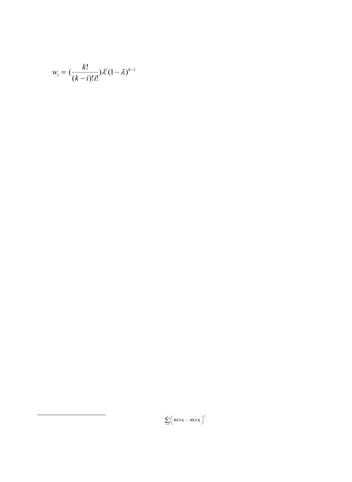
where
λ
is the binomial parameter.
The regression model for performance (return on assets) can thus be stated as:
ROA
it
=
b
1
Exploitation
+
b
2
Prior Exploitation
+
b
3
Exploitation
+
b
4
Controls
+
ɛ
(3)
The introduction of the parameter
λ
added one degree of freedom to the model. By
minimizing the sum of the squared residuals,
3
an optimal
λ
could be found. As a result, the
distribution of
W
i
and the lag structure of
Prior Exploration
could be determined.
A multivariate linear regression procedure was then adopted. The model takes account
of both time and firm-specific fixed effects to control for unobservable effects. Following
Ravenscraft and Scherer (1982), we set
k
= 8,
4
i.e., the lag period was from
t
-8 to
t
-1.
4. Results
By minimizing the sum of the squared residuals in equation (3), the optimal value for
λ
was found to be 0.2680. Substituting
λ
into equation (2), we calculated the values for w
0
to
w
7
as 0.0824, 0.2414, 0.3094, 0.2265, 0.1037, 0.0304, 0.0056 and 0.0006, respectively. The
value for
prior exploration
was thus derived from equation (1).
This result presents a bell-shaped exploration distribution with more of the lag effect
found between year 2 (weighted by w
1
) and year 5 (weighted by w
4
), suggesting that the time
lag between the beginning of exploratory investments and the commercialization of such
investments in the semiconductor industry was 2 to 5 years. This finding is consistent with
evidence from prior studies as well as field experience. Previous research has found that for
the two-digit SIC electrical and electronics industry (SIC 36), the lag period for having a
major impact is about 3 to 5 years (Lev and Sougiannis, 1996). The semiconductor industry
is one of the most technology-intensive of the SIC 36 industries. Thus, a relatively long lag
period, such as the 3 to 5 years is to be expected. As predicted by the famous Moore’s Law,
3 The sum of squared residuals was calculated as
4 We also tested multivariate linear regression results for k = 6 and k = 7, these robustness tests produce
consistent results; the sign and significance of variables were unchanged.


